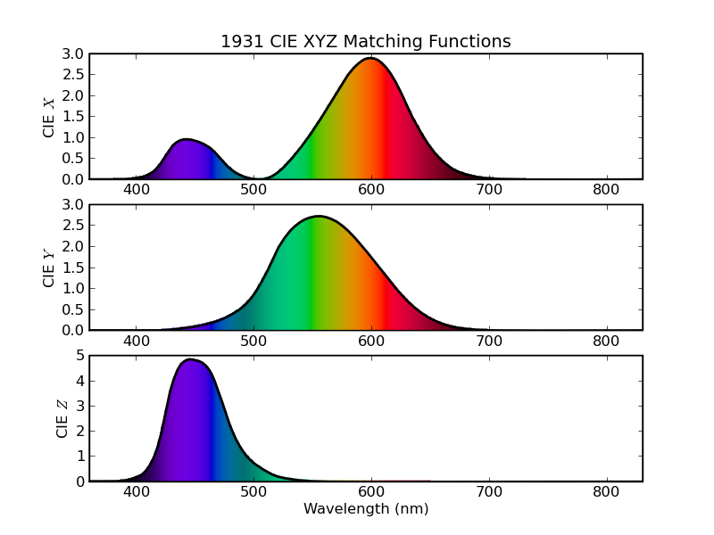
Figure 1 - The 1931 CIE XYZ matching functions.
ColorPy is a Python package that can convert physical descriptions of light - spectra of light intensity vs. wavelength - into RGB colors that can be drawn on a computer screen. It provides a nice set of attractive plots that you can make of such spectra, and some other color related functions as well. All of the plots in this documentation were created with ColorPy.
ColorPy is free software. ('Free' as in speech and beer.) It is released under the GNU Lesser GPL license. You are free to use ColorPy for any application that you like, including commercial applications. If you modify ColorPy, you should release the source code for your modifications. You have no obligation to release any source for your products that just use ColorPy, however.
Several years ago, I developed some C++ code to do these kinds of physical color calculations. Recently, I decided to port the code to Python, and publish the library as open source under the GNU LGPL license. I decided to make use of (and assume the existence of) NumPy and MatPlotLib for this. These libraries make it easy to make some nice, attractive, and informative, plots of spectra. Besides, Python is just more fun than C++.
So what can ColorPy do? The short answer, is to scan this document, and examine the various plots of spectra and their colors. You can use ColorPy to make the same kinds of plots, for whatever spectra you have and are interested in. ColorPy also provides conversions between several important three-dimensional 'color spaces', specifically RGB, XYZ, Luv, and Lab. (There can be many different RGB spaces, depending on the particular display used to view the results. By default, ColorPy uses the sRGB space, but you can configure it to use other RGB spaces if you like.)
Copyright (C) 2008 Mark Kness
Author - Mark Kness - mkness@alumni.utexas.net
ColorPy is free software: you can redistribute it and/or modify it under the terms of the GNU Lesser General Public License as published by the Free Software Foundation, either version 3 of the License, or (at your option) any later version. ColorPy is distributed in the hope that it will be useful, but WITHOUT ANY WARRANTY; without even the implied warranty of MERCHANTABILITY or FITNESS FOR A PARTICULAR PURPOSE. See the GNU Lesser General Public License for more details. You should have received a copy of the GNU Lesser General Public License along with ColorPy. If not, see http://www.gnu.org/licenses/.
To use ColorPy, you must have installed the following: Python, NumPy, and MatPlotLib. Typically, SciPy is installed along with NumPy and MatPlotLib. ColorPy doesn't use SciPy explicitly, although MatPlotLib may require SciPy. (I am not sure.) ColorPy is a 'pure' Python distribution, so you do not need any extra software to build it. I have tested ColorPy both on Windows XP and Ubuntu Linux, and it should run on any system where you can install the prerequisites. If, for some reason, you can only install NumPy but not MatPlotLib, you should still be able to do many of the calculations, but will not be able to make any of the nice plots.
ColorPy generally uses wavelengths measured in nanometers (nm), 10-9 m. Otherwise, typical metric units are used. For descriptions of spectra, ColorPy uses two-dimensional NumPy arrays, with two columns and an arbitrary number of rows. Each row of these arrays represents the light intensity for one wavelength, with the value in the first column being the wavelength in nm, and the value in the second column being the light intensity at that wavelength. ColorPy can provide a blank spectrum array, via colorpy.ciexyx.empty_spectrum(), which will have rows for each wavelength from 360 nm to 830 nm, at 1 nm increments. (Wavelengths outside this range are generally ignored, as the eye cannot see them.) However, you can create your own spectrum arrays with any set of wavelengths you like.
Color values are represented as three-component NumPy vectors. (One-dimensional arrays). Typically, these are vectors of floats, with the exception of displayable irgb colors, which are arrays of integers (in the range 0 - 255).
We are interested in working with physical descriptions of light spectra, that is, functions of intensity vs. wavelength. However, color is perceived as a three-dimensional quantity, as there are three sets of color receptors in the eye, which respond approximately to red, green and blue light. So how do we reduce a function of intensity vs. wavelength to a three-dimensional value?
This fundamental step is done by integrating the intensity function with a set of three matching functions. The standard matching functions were defined by the Commission Internationale de l'Eclairage (CIE), based on experiments with viewers matching the color of single wavelength lights. The matching functions generally used in computer graphics are those developed in 1931, which used a 2 degree field of view. (There is also a set of matching functions developed in 1964, covering a field of view of 10 degrees, but the larger field of view does not correspond to typical conditions in viewing computer graphics.) So the mapping is done as follows:
X = ∫ I (λ) * CIE-X (λ) * dλ
Y = ∫ I (λ) * CIE-Y (λ) * dλ
Z = ∫ I (λ) * CIE-Z (λ) * dλ
where I (λ) is the spectrum of light intensity vs. wavelength, and CIE-X (λ), CIE-Y (λ) and CIE-Z (λ) are the matching functions. The CIE matching functions are defined over the interval of 360 nm to 830 nm, and are zero for all wavelengths outside this interval, so these are the bounds for the integrals.
So what do these matching functions look like? Let's take a look at a plot (made with ColorPy, of course.)
Figure 1 - The 1931 CIE XYZ matching functions.
This plot shows the three matching functions vs. wavelength. The colors underneath the curve, at each wavelength, are the (approximate) colors that the human eye will perceive for a pure spectral line at that wavelength, of constant intensity. The apparent brightness of the color at each wavelength indicates how strongly the eye perceives that wavelength - the intensity for each wavelength is the same. (The next section will explain how we get the RGB values for the colors.)
Each of the three plots was generated via colorpy.plots.spectrum_subplot (spectrum), where spectrum is the value of the matching function vs. wavelength.
All three of the matching functions are zero or positive everywhere. Since the light intensity at any wavelength is never negative, this means that the resulting XYZ color values are never negative. Also, the Y matching function corresponds exactly to the luminous efficiency of the eye - the eye's response to light of constant luminance. (These facts are some of the reasons that make this particular set of matching functions so useful.)
So now we can map a spectrum of intensity vs. wavelength into a three-dimensional value. Before we consider how to convert this into an RGB color value that we can draw, we will first discuss some typical scaling operations on XYZ colors.
Often, it is useful to consider the 'chromaticity' of a color, that is, the hue and saturation, independent of the intensity. This is typically done by scaling the XYZ values so that their sum is 1.0. The resulting scaled values are conventionally written as lower case letters x,y,z. With this scaling, x+y+z = 1.0. The chromaticity can be specified by the resulting x and y values, and the z component can be reconstructed as z = 1.0 - x - y. It is also common to specify colors with their chromaticity (x and y), as well as the total brightness (Y). Occasionally, one also wants to scale an XYZ color so that the resulting Y value is 1.0.
ColorPy represents XYZ colors (and other types of colors) as three-component vectors. There are some 'constructor' like functions to create such arrays, and perform these kinds of scaling:
colorpy.colormodels.xyz_color (x, y, z = None)
colorpy.colormodels.xyz_normalize (xyz)
colorpy.colormodels.xyz_color_from_xyY (x, y, Y)
colorpy.colormodels.xyz_normalize_Y1 (xyz)
Notice that color types are generally specified in ColorPy with lower case letters, as this is more readable. (I.e., xyz_color instead of XYZ_color.) The user must keep track of the particular normalization that applies in each situation.
So how do we convert one of these XYZ colors to an RGB color that I can draw on my computer?
The short answer, is to call colorpy.colormodels.irgb_from_xyz (xyz), where xyz is the XYZ color vector. This will return a three element integer vector, with each component in the range 0 - 255. There is also a function colorpy.colormodels.irgb_string_from_xyz (xyz) that will return a hex string, such as '#FF0000' for red.
There are several subtleties and approximations in the behavior of these functions, which are important to understand what is happening.
The first step in the conversion, is to convert the XYZ color to a 'linear' RGB color. By 'linear', we mean that the light intensity is proportional to the numerical color values. ColorPy represents such linear RGB values as floats, with the nominal range of 0.0 - 1.0 covering the range of intensity that the monitor display can produce. (This implies an assumption as to the physical brightness of the display.) The conversion from XYZ to linear RGB is done by multiplication by a 3x3 element array. So, which array to use? The specific values of the array depend on the physical display in question, specifically the chromaticities of the monitor phosphors. Not all displays have the exact same red, green and blue monitor primaries, and so any conversion matrix cannot apply to all displays. This can be a considerable complication, but fortunately, there is a specification of monitor chromaticities that we can assume, part of the sRGB standard, and are likely to be a close match to most actual displays. ColorPy uses this assumption by default, although you can change the assumed monitor chromaticities to nearly anything you like.
So for now, let's assume the standard sRGB chromaticities, which gives us the correct 3x3 matrix, and so we can convert our XYZ colors to linear RGB colors.
We then come to the next obstacle... The RGB values that we get from this process are often out of range - meaning that they are either greater than 1.0, or even that they are negative! The first case is fairly straightforward, it means that the color is too bright for the display. The second case means that the color is too saturated and vivid for the display. The display must compose all colors from some combination of positive amounts of the colors of its red, green and blue phosphors. The colors of these phosphors are not perfectly saturated, they are washed out, mixed with white, to some extent. So not all colors can be displayed accurately. As an example, the colors of pure spectral lines, all have some negative component. Something must be done to put these values into the 0.0 - 1.0 range that can actually be displayed, known as color clipping.
In the first case, values larger than 1.0, ColorPy scales the color so that the maximum component is 1.0. This reduces the brightness without changing the chromaticity. The second case requires some change in chromaticity. By default, ColorPy will add white to the color, just enough to make all of the components non-negative. (You can also have ColorPy clamp the negative values to zero. My personal, qualitative, assessment is that adding white produces somewhat better results. There is also the potential to develop a better clipping function.)
So now we have linear RGB values in the range 0.0 - 1.0. The next subtlety in the conversion process, is that the intensity of colors on the display is not simply proportional to the color values given to the hardware. This situation is known as 'gamma correction', and is particularly significant for CRT displays. The voltage on the electron gun in the CRT display is proportional to the RGB values given to the hardware to display, but the intensity of the resulting light is *not* proportional to this voltage, in fact the relationship is a power law. The particular correction for this depends on the physical display in question. LCD displays add another complication, as it is not clear (at least to me) what the correct conversion is in this case. Again, we rely on the sRGB standard to decide what to do. That standard assumes a physical 'gamma' exponent of about 2.2, and ColorPy applies this correction by default. You can change this to a different exponent if you like.
The final step after gamma correction, is to convert the RGB components from the range 0.0 - 1.0 to 0 - 255, which is the typical range needed to pass to the hardware. This is done with simple scaling and rounding. The final result of all of these conversions, RGB color values in the range 0 - 255, is referred to as an irgb_color. This is the color type that can be passed to drawing functions.
Summarizing of these conversions, with the functions that ColorPy uses internally:
colorpy.colormodels.rgb_from_xyz (xyz) - Converts an XYZ color to a linear RGB color, with components in the nominal range 0.0 - 1.0, but possibly out of range (greater than 1.0, or negative). The resulting linear RGB color cannot be directly passed to drawing functions.
colorpy.colormodels.irgb_from_rgb (rgb) - Converts a linear RGB color in the nominal range 0.0 - 1.0 to a displayable irgb color, definitely in the range 0 - 255. Color clipping may be applied (intensity as well as chromaticity), and gamma correction is accounted for. This result can be passed to drawing functions.
With all of this, let's plot some real colors. First, consider the pure spectral lines - that is, spectra that are all black (zero intensity), except at a single wavelength. We consider all the wavelengths from 360 nm to 830 nm, which covers the range of human vision (and the range of the CIE XYZ matching functions.)
The two-part plot below shows the result. The top section, shows the best colors that ColorPy can draw for each wavelength. The amount of light intensity for each wavelength is the same. But since the human eye has different sensitivity to different wavelengths, the apparent brightness looks different for different colors. For example, the color for 750 nm is quite dark, while the color for 550 nm is quite bright. They represent lines with the same physical luminance, however. The bottom section shows the linear RGB values corresponding to each wavelength. You can see that there are negative RGB values on this plot. In fact, there is a negative component at every wavelength - none of the pure spectral lines can be displayed with full saturation. (The overall intensity scale is arbitrary, and has been chosen so that the largest RGB component for any wavelength is 1.0.)

Figure 2 - RGB values for the pure spectral lines.
This specific plot was made with colorpy.plots.visible_spectrum_plot (), and the real work was done with colorpy.plots.color_vs_param_plot (param_list, rgb_colors, title, filename, tight=False, plotfunc=pylab.plot, xlabel='param', ylabel='RGB Color'). This function accepts two lists, one of an arbitrary parameter (wavelength in this case), and one of linear RGB colors. (The two lists must be of the same size.) You also must supply a title and filename for the plot. Optional arguments include a request that the x-axis be 'tightened' to only include the range of the parameters, a different plotting function from the default, and different labels for the axes. This is a very handy function, useful for many other plots besides this one.
You can see that there are negative RGB values for these colors, and those actually drawn have been clipped to something displayable.
Another way to understand the limited color gamut (range of displayable colors) of physical displays, is to consider the 'shark fin' CIE chromaticity diagram. On this plot, we draw the chromaticities of the pure spectral lines. These trace out a fin shaped region. The low wavelength colors start at the lower left corner of the fin, and as the wavelength increases, moves up on the plot towards green, and then down and to the right towards yellow and red. The longest wavelength corresponds to the red corner at the far right. The straight line connecting the long wavelength red to the short wavelength blue is not composed of pure spectral lines, rather these 'purples' are a linear combination of the extreme red and blue colors. The outer boundary of this diagram represents the spectrally pure colors. Just inside this boundary, we draw the best color match for each wavelength.
The triangle inside the fin represents the range (gamut) of colors that the physical display can show. The vertices labeled Red, Green and Blue represent the chromaticities of the monitor primaries, and the point labeled White represents the white point with all primaries at full strength. (This plot assumes the standard sRGB primaries and white point.) The points inside the inner triangle are the only colors that the display can render accurately. (This figure could use a little work. It would be nice to label the outer boundary of the fin with the corresponding wavelength.) The points outside the inner triangle are colors that must be approximated. (Points outside the outer 'fin' do not correspond to any color at all.)
You can see that the standard monitor is much more limited in displaying greens than blues and reds. If someone is able to invent a much purer green colored phosphor, with low persistence so it is suitable for animations and hence real displays, then the world of computer graphics will get significantly more richly colored! Also notice that there is no possible set of of three monitor phosphor chromaticities that can cover the entire visible gamut. For any three points inside the 'fin', the enclosed triangle must necessarily exclude some of the pure spectral colors, even if the monitor phosphors were perfectly spectrally pure.
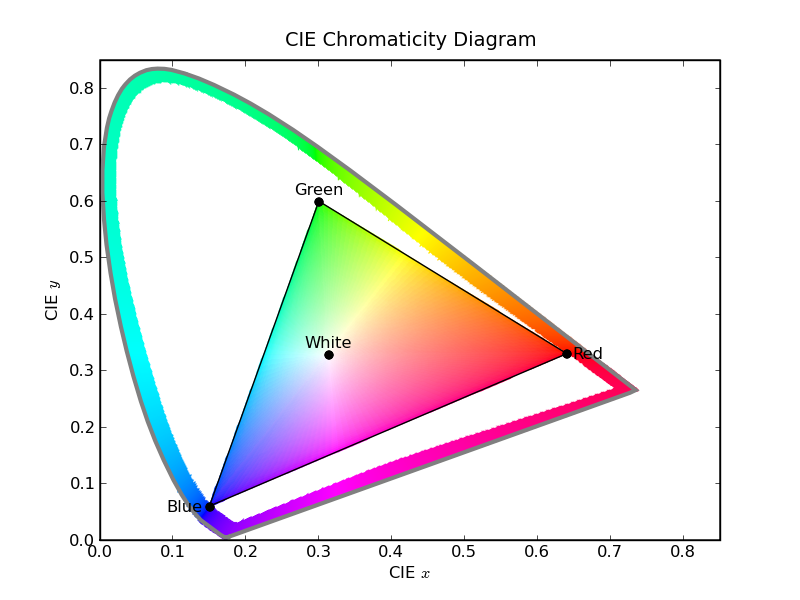
Figure 3 - CIE chromaticity diagram of the visible gamut.
Colors inside
the inner triangle can be accurately drawn on the display, points outside (but
inside the fin) must be approximated.
This figure is drawn with colorpy.plots.shark_fin_plot(). This is kind of a specialized figure, probably not that useful for other things. Now, let's consider some more examples.
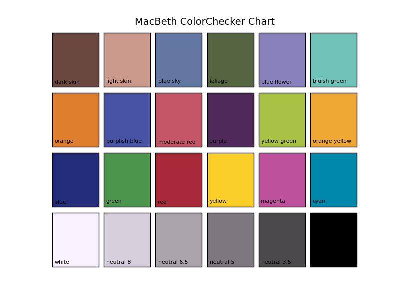
Figure 4 - MacBeth ColorChecker Chart.
The simplest way that ColorPy can be used to display colors, is to display a set of known XYZ (or RGB) colors. As an example, we use the MacBeth ColorChecker Chart. This is a set of standard reference colors that is used in photography and video. (You can buy the physical chart from photographic suppliers. It is not particularly cheap.) It is used to verify that colors are being reproduced accurately on film. [Hall, p. 119] provides a set of xy colors for the patches on this chart (which must assume some particular lighting environment), and ColorPy can convert these into displayable colors. This serves as a test that the xyz to rgb conversions are operating correctly, which is analogous to the sort of thing the real chart is used for.
This 'patch' plot is made with colorpy.plots.xyz_patch_plot (xyz_colors, color_names, title, filename, patch_gap=0.05, num_across=6), where xyz_colors and color_names are two lists, the first with the XYZ color values to draw, and the second with names to draw on the plot. The two lists must be of the same size, but you can pass None for the second list to skip the labels. You also must supply a title and filename, and there are optional arguments to fine-tune the size and arrangement of the patches. There is also a similar function colorpy.plots.rgb_patch_plot() when you have known RGB values that you want to draw.
For a more interesting example, one that involves physical light spectra, consider the colors of thermal blackbodies. A 'blackbody' is an object that is in thermal equilibrium with its environment, at some temperature T. Such an object will radiate light energy, with a particular spectrum of intensity vs. wavelength. This spectrum depends only on the temperature of the blackbody, and is completely independent of the composition of the blackbody. The theory of blackbodies was important in the development of quantum mechanics, the first application of quantum mechanics was by Max Planck in deriving the blackbody spectrum. Many real light sources are approximately blackbodies.
Blackbody theory shows that the 'monochromatic specific intensity' Bλ(T), the power at wavelength λ radiated per unit wavelength per unit solid angle, is [Shu p. 78]:
Bλ(T) = (2hc2)/(λ5) * (1 / (exp(hc/λkT) - 1))
where h = Planck's constant, c = speed of light, k = Boltzman's constant, λ = wavelength, and T = temperature.
Using this relation, we can construct a spectrum in ColorPy, and then determine the rgb color of the blackbody radiator. The module blackbody provides the appropriate functions. First, the function blackbody.blackbody_specific_intensity (wl_nm, T_K) calculates the Bλ(T) above, for any wavelength and temperature. This is then converted into a spectrum of intensity vs. wavelength. The function ciexyz.empty_spectrum() is called to get a NumPy array to hold the spectrum. This array has one row for each wavelength to be used, from 360 to 830 nm, with an increment of 1 nm. The first column is already filled in with the wavelength (in nm), the second column is to be filled with the intensity, and is initially zero. Since Bλ(T) represents the power per unit wavelength, this must be multiplied by the width of the interval, which is 1 nm. This resulting spectrum is then converted into an xyz color with ciexyz.xyz_from_spectrum(). This can then be converted to a displayable irgb color and drawn. The whole process is performed by colorpy.blackbody.blackbody_spectrum(), which is listed below.
def blackbody_spectrum (T_K):
'''Get the spectrum of a blackbody, as a numpy array.'''
spectrum = ciexyz.empty_spectrum()
(num_rows, num_cols) = spectrum.shape
for i in xrange (0, num_rows):
specific_intensity = blackbody_specific_intensity (spectrum [i][0], T_K)
# scale by size of wavelength interval
spectrum [i][1] = specific_intensity * ciexyz.delta_wl_nm * 1.0e-9
return spectrum
So let's look at some results of these calculations, which also introduce a new type of ColorPy plot, the spectrum plot. First, consider a blackbody with a temperature of 5778 K. This is the surface temperature of the Sun [Wikipedia], and this spectrum approximates that of the sun. Figure 5 below shows both the overall color of the resulting spectrum, with a graph of the spectrum itself below the color patch. The overall color is nearly white. The spectrum shows that the peak intensity is in the green region, around 500 nm or so, but with significant contributions from both lower and higher wavelengths. The colors in the spectrum plot are indicate the extent to which the eye is sensitive to the particular wavelength. Each color band has the same amount of luminance, so the apparent brightness of the color indicates the extent to which the eye is sensitive to that wavelength. The eye has a very low sensitivity to wavelengths below 400 nm or so, and to wavelengths above 700 nm or so. Thus, the resulting color in the spectrum plot is nearly black. With a wavelength of 550 nm, on the other hand, the eye is quite sensitive to this wavelength, and the resulting color is therefore bright (green). This way of drawing the spectrum is intended to help show the contributions of each wavelength in the spectrum to the overall color. For example, in this case, there is a considerable amount of power at wavelengths from 700 nm to 830 nm. However, the eye has a low sensitivity to these, and so these wavelengths do not contribute much to the overall color.
These kinds of plots are made with colorpy.plots.spectrum_plot (spectrum, title, filename, xlabel, ylabel), where spectrum is the numpy array with the spectrum data, and the other parameters are the title, filename, and axis labels.
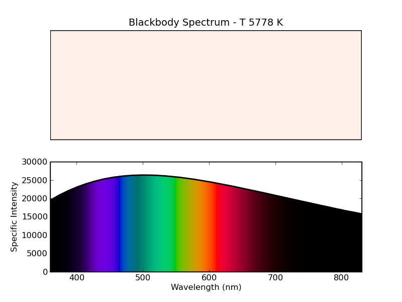
Figure 5 - Color of a 5778 K blackbody. This approximates the spectrum of
the Sun.
Since the temperature is just a parameter to the function calls, we can do the same thing for any other temperature that we like. The nearby star Proxima Centauri is much cooler than the sun, it has a surface temperature of about 3000 K. [Wikipedia]. The spectrum of a 3000 K blackbody is shown below, with the same kind of plot. The overall color in this case is orange, and the spectrum is concentrated at longer wavelengths.
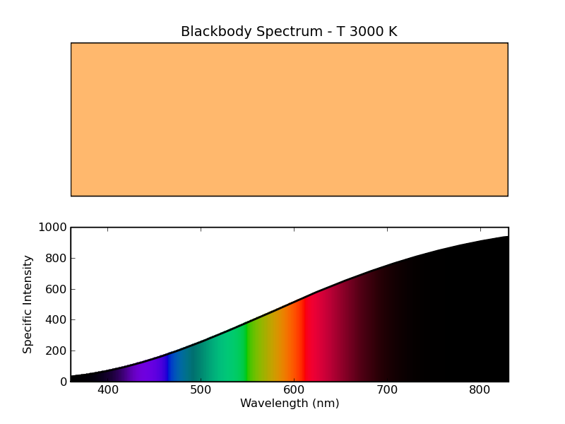
Figure 6 - Spectrum of 3000 K blackbody. This approximates the spectrum of Proxima Centauri.
We can also evaluate this at higher temperatures. The star Rigel, in the constellation Orion, has a surface temperature of 11000 K [Wikipedia], and the resulting blackbody spectrum is shown below. The overall color is now blue-white, and the intensity is concentrated at low wavelengths.
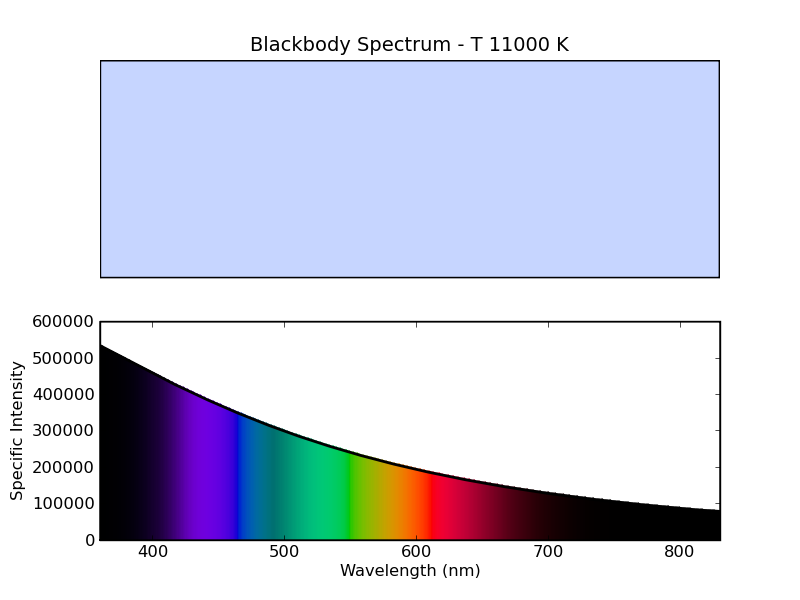
Figure 7 - Spectrum of 11000 K blackbody. This approximates the spectrum
of the star Rigel.
But why limit ourselves to just a handful of temperatures? We can calculate the blackbody spectrum for very many temperatures, and ColorPy allows us to plot the resulting color vs. temperature, while also showing a plot of the rgb color values. In the figure below, we have calculated the blackbody color for temperatures ranging from 1200 K to 16000 K. The top subplot shows the resulting color, as a function of temperature, while the lower plot shows the linear RGB values. For low temperatures, the blackbody is red to orange, and as the temperature increases, the color becomes white, and then blue.
This style plot was generated with colorpy.plots.color_vs_param_plot (param_list,
rgb_colors, title, filename, tight, plotfunc, xlabel, ylabel). The
arguments tight, plotfunc, xlabel and ylabel are optional, in this case we set
tight=True and plotfunc=pylab.semilogy to obtain the semilog plot, which is
needed for the very large range of color values covered.
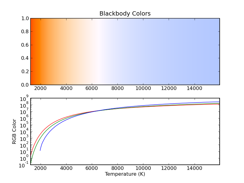
Figure 8 - Color of blackbody vs. temperature.
Let's also consider similar plots over different temperature ranges. First, consider the range 950 K to 1200 K, shown below. The colors are all nearly red, and are brighter for higher temperatures.
This provides another example to discuss the color intensity scaling that ColorPy uses. ColorPy attempts to calculate a color value that, when displayed on a computer monitor, will match the physical brightness of the spectrum. In this plot, the red value reaches 1.0 at about 1150 K. This means (approximately) that an 1150 K blackbody is as bright as the monitor at full intensity. Similarly, a 950 K blackbody is about 1.5% as bright as the monitor. This, by the way, suggests an experimental test of whether the display brightness assumed by ColorPy is correct - a 1150 K blackbody is predicted to be as bright as the display monitor at full red.
Also notice that there is no blue line on this plot. For temperatures as low as 1200 K (and all lower), the correct blue value is negative. (This means that the monitor is not capable of displaying the color at full saturation - it is necessarily washed out.) Since negative values cannot be plotted on a log axis, there is no blue on this plot. The green value also becomes negative near the left edge of the plot.
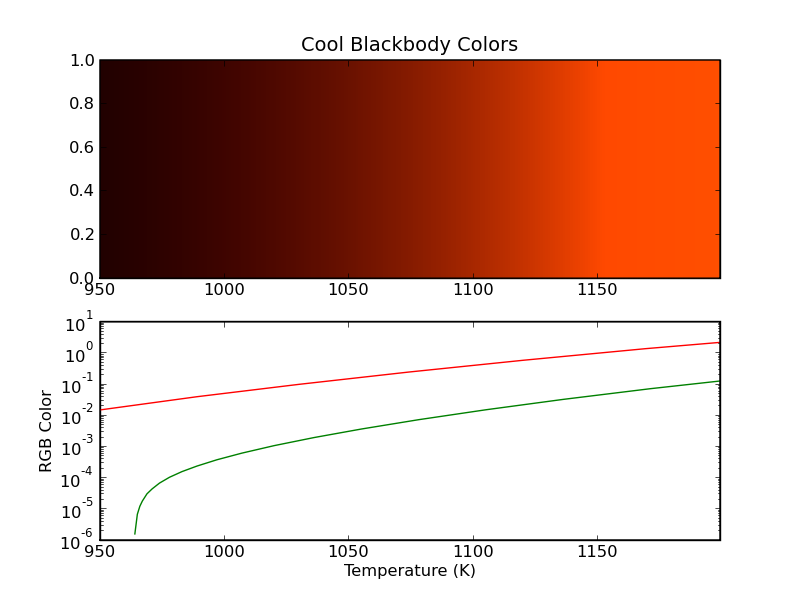
Figure 9 - Colors of relatively cool blackbodies.
Now consider a high temperature range, 10000 K to 40000 K, shown in the plot below. In this situation, the colors are far in excess of that displayable on the monitor. A 40000 K blackbody is far far brighter than any computer monitor! In fact, the intensity is on the order of 109 times that of what the monitor can display. When displaying very bright colors such as this, ColorPy will scale them to the brightest color, of the same hue and saturation, that can be displayed. In this case, where all the colors are scaled like this, the resulting RGB values all have similar brightness. So, all the colors on this chart are of similar brightness. However, there is actually a large range in physical brightness - a 40000 K blackbody is much brighter than a 10000 K blackbody. Note how this contrasts with the situation on the cool blackbody plot, where the intensity of the displayed colors varied with temperature. There is a physical variation in intensity in both cases, but ColorPy can only show this when the colors are in the range displayable by the monitor.
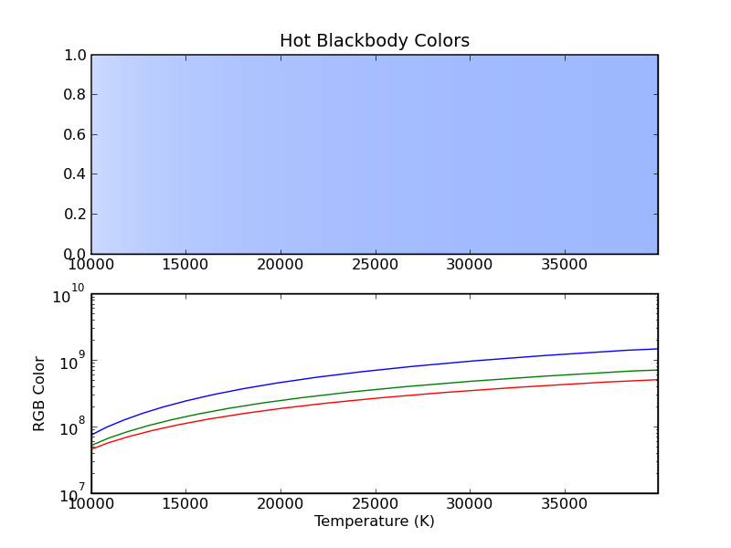
Figure 10 - Colors of relatively hot blackbodies.
For a second example, consider Rayleigh scattering. This concerns the scattering of light by small particles (much smaller than the wavelength of the light.) In this situation, the amount of scattering is inversely proportional to the fourth power of the wavelength. To compute the spectrum resulting from Rayleigh scattering, we need a description of the original light source, the 'Illuminant', as the power emitted as a function of wavelength. Then, the spectrum resulting from Rayleigh scattering is [van de Hulst, p. 65]:
Scattered Intensity (λ) = Illuminant (λ) * a * (1 / λ4)
where a is a proportionality constant. (In the plots below, we have arbitrarily taken the constant a so that the value of the Rayleigh scattering term at 550 nm is 1.0.)
Often, the intensity of the illuminant is arbitrary. The illuminants provided by ColorPy are scaled so that they have Y = 1.0, which means that they are about as bright as the monitor at full white. One obvious choice for an illuminant is a blackbody. ColorPy will provide an illuminant for a blackbody of any temperature you like, with colorpy.illuminants.get_blackbody_illuminant (T_K). (Remember that these illuminants are scaled to have a Y = 1.0, rather than the (typically) much larger brightness of a true blackbody.)
A familiar illuminant is the one for a 5778 K blackbody, which approximates the illumination of the Sun. The plot below shows the effect of Rayleigh scattering of this illuminant. The overall color is sky blue, with the spectrum concentrated at low wavelengths. This result is as expected, as Rayleigh scattering is the basic physical reason that the sky is blue.
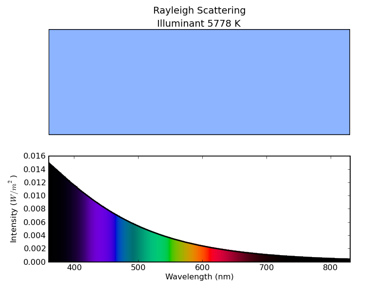
Figure 11 - Rayleigh scattering of a 5778 K blackbody. Why the sky is blue.
But why limit ourselves to the color of our Sun? With ColorPy, we can do the same calculations for a blackbody of any temperature we like. So we repeat the process, first for a temperature of 3000 K (Proxima Centauri), and then for a temperature of 11000 K (Rigel). The plots below show the results. If we lived on a planet around Proxima Centauri, the sky would be nearly white. On the other hand, if we lived on a planet near Rigel, the sky would also be blue, but a deeper shade of blue than we have on Earth.
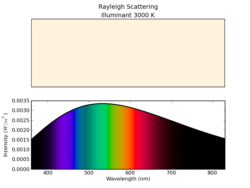
Figure 12 - Rayleigh scattering of a 3000 K blackbody. The color of the sky
from near Proxima Centauri.

Figure 13 - Rayleigh scattering of a 11000 K blackbody. The color of the
sky from near Rigel.
We can also make a plot for many temperatures, and get a plot of the color of the sky vs. blackbody illuminant temperature, similar to the plot we made of the color of the blackbody itself vs. temperature. The range of sky colors is about the same as the range of blackbody colors, but the sky colors are bluer than the blackbody colors, for any given temperature.
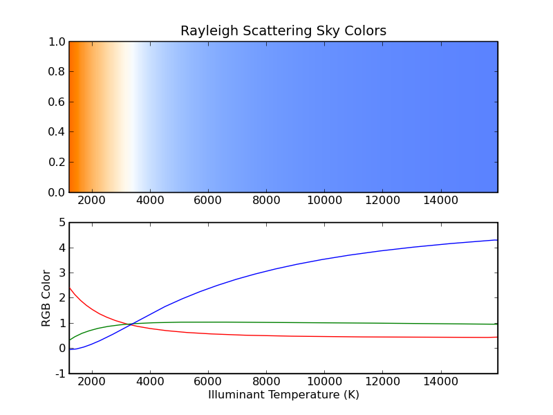
Figure 14 - Color of the sky for various temperature blackbody illuminants.
ColorPy provides several different 'illuminant' functions that can be used as light sources. In addition to the blackbody illuminants, ColorPy provides the CIE standard Illuminant D65. Illuminant D65 is intended to provide a good approximation for normal daylight. Illuminant D65 is recommended as the general-purpose, default, illumination for daytime conditions (on Earth only however!)
Illuminant D65 is given by a table of intensity vs. wavelength, rather than a mathematical formula. ColorPy provides this illuminant, normalized so that Y = 1.0, as usual. The spectrum of D65 is shown below. Note that the overall color is white. In fact, D65 is used as the white point for determining the xyz to rgb conversion matrix, so D65 is in fact the very definition of white!
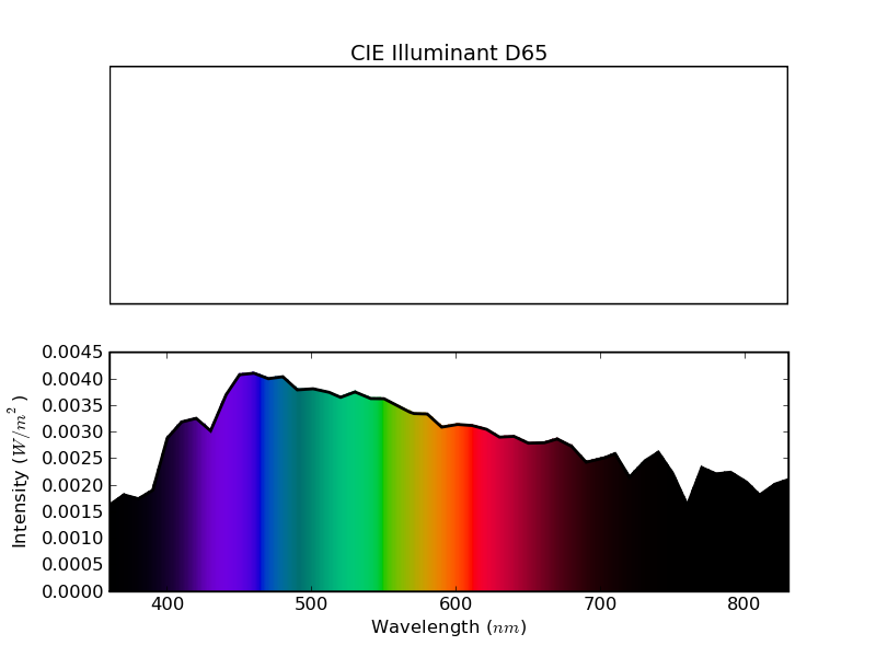
Figure 15 - Spectrum of CIE Illuminant D65.
In this example, we will calculate the colors produced by interference films, such as a soap bubble, or an oil slick on water. This time, we will use D65 as the illuminant.
The physical situation can be described by illumination from above, passing through a dielectric medium with some index of refraction n1. As the wave propagates, it meets an interface where the index of refraction changes to a new value n2. At the interface, part of the original wave is reflected, and part continues into the new medium. The material n2 is considered to be in a thin layer. After passing through this thin layer, the wave meets a second interface, where the index of refraction changes from n2 to n3. Again, part of the incident wave is reflected from the interface, and part continues to propagate.
We will assume that the regions where the index is n1 and n3 are infinite in extent, while the region where the index is n2 is limited to a thin layer, with thickness t.
Some typical indices of refraction of real materials are:
n = 1.000 - Vacuum
n = 1.003 - Air
n = 1.33 - Water
n = 1.44 - Oil
n = 1.50 - Glass
The total reflected wave from the system is a combination of the wave reflected from the first interface (n1 to n2), and the wave reflected from the second interface (n2 to n3).
There may be multiple reflections - e.g. the wave reflected from the second interface will not fully pass through the (now reversed) interface from n2 to n1, rather only part will pass, while some will reflect again and head back to the interface from n2 to n3. The calculations in ColorPy consider all numbers of multiple reflections, not just a single reflection.
What makes the interesting colors, is that the two waves travel through a different path length, and this results in them being out of phase. The exact change in phase depends on both the wavelength of the light, the thickness of the layer, and the index of refraction of the layer. Depending on the specifics, the two waves may constructively interfere, resulting in a large amplitude of the reflected wave, or the waves may destructively interfere, resulting in a small (or zero) amplitude of the reflected wave, or something in between.
Whether the interference is constructive or destructive depends on the wavelength, and for thin films, part of the spectrum will be reduced from destructive interference, and part enhanced from constructive interference, resulting in a significant color shift.
First, consider a soap bubble. In this situation, material 1 is air, material 2 is a solution of soap in water, while material 3 is air again. (The inside of the bubble.) So, n1 = 1.003, n2 = 1.33, and n3 = 1.003. Calculating the color of the total reflection, with an illuminant of D65, as a function of the thickness of the layer, results in the plot below. Note that the RGB components oscillate as the thickness is varied.
The phase relationship between the red, green and blue components affects the resulting color.
For the most part, these stay within the displayable range of 0.0 to 1.0, but there are a few places where the red component becomes negative, in the most vivid green regions. These vivid green colors cannot be properly displayed on the monitor, the true color is more saturated than what is shown. Most of the other colors can be displayed properly.
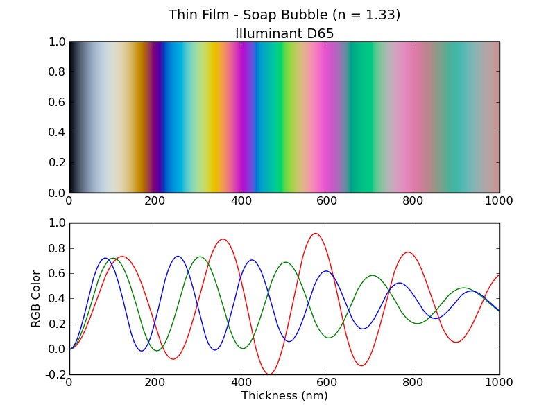
Figure 16 - Color of reflections from a soap bubble. The illuminant is D65.
For a particular thickness of the film, we can plot the reflectance spectrum. The plots below show the spectrum for some of the particularly vivid colors, for thicknesses (not wavelengths!) of 400 nm and 500 nm. For these plots, we used an illuminant that is constant over wavelength, rather than D65. The only reason is to avoid the jaggedness of the D65 curve from making the plot more confusing.
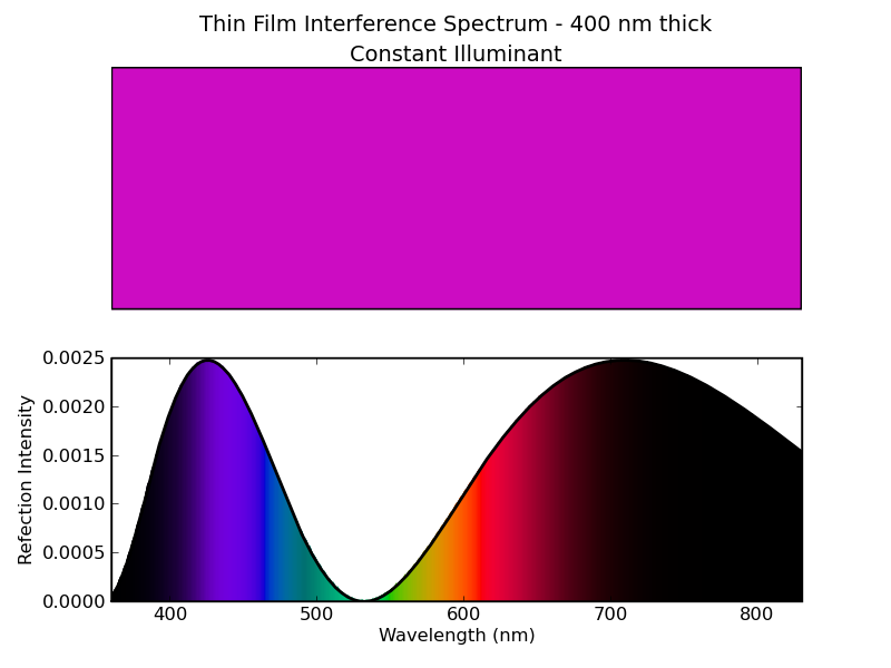
Figure 17 - Spectrum of soap bubble reflection for a thickness of 400 nm.
The illuminant is constant over wavelength.
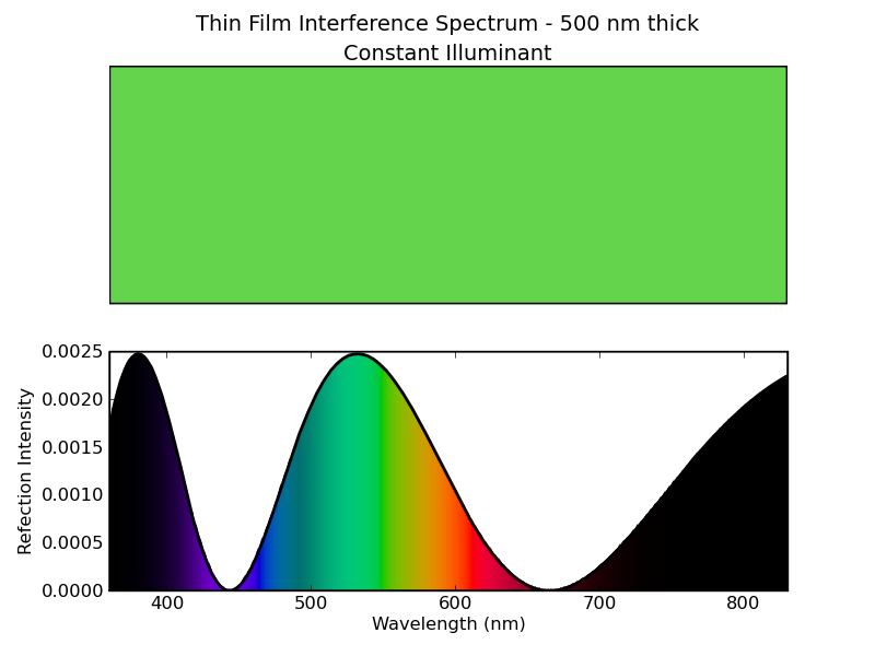
Figure 18 - Spectrum of soap bubble reflection for a thickness of 500 nm.
The illuminant is constant over wavelength.
We can do the same thing for an oil slick floating on water. In this case, medium 1 is air (n = 1.003), medium 2 is oil (n = 1.44), and medium 3 is water (n = 1.33). The result is shown below. Note that the colors are not as saturated and vivid as for the reflection from a soap bubble. Since these colors are less saturated than the soap bubble reflections, all of them are properly displayable on the computer.
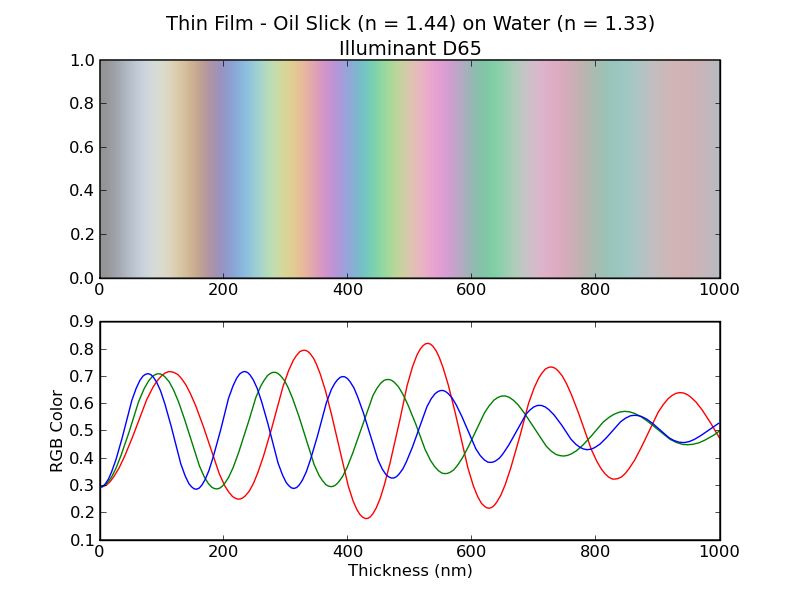
Figure 19 - Color of reflections from an oil slick. The illuminant is D65.
ColorPy also provides some color manipulation functions, that are not directly related to physical color calculations. The most important of these are routines to convert colors into the nearly perceptually uniform color spaces Luv and Lab.
The common color spaces rgb and xyz are not very perceptually uniform. This means that, if you calculate the distance between two colors C1 and C2, using the usual Euclidean metric, namely:
Distance = √ ((Red2 - Red1)2 + (Green2 - Green1)2 + (Blue2 - Blue1)2)
the calculated distance values do not agree well with the psychological apparent differences in the colors. I.e., the mind may see two colors as very different, but where they have a small distance, or alternately the mind may see two colors as similar, but where they have a large color distance. This causes difficulties in calculating the 'closest color'. (Since xyz and rgb values are linearly related, the same distance issues apply to both of those spaces.)
The color spaces Luv and Lab are designed to be a much more perceptually uniform color space than rgb or xyz. If colors are transformed into Luv or Lab space, then mathematical distance calculations, using the Euclidean metric, on Luv and Lab values will provide a much better assessment of how different the colors appear.
These perceptually uniform color spaces are not perfect. (The fact that there are two of them, is a clear sign that they are imperfect.) However, they should do a substantially better job in measuring the apparent differences in colors.
ColorPy provides routines to transform color values from xyz into both Luv and Lab, and also routines to convert back to xyz. Coupled with the conversions between xyz and rgb, one can convert between any of the desired color spaces. Most descriptions of the Luv and Lab models only provide the transformation from xyz to Luv and Lab, but ColorPy also provides the inverses. The conversion routines are:
colorpy.colormodels.luv_from_xyz (xyz)
colorpy.colormodels.xyz_from_luv (luv)
colorpy.colormodels.lab_from_xyz (xyz)
colorpy.colormodels.xyz_from_lab (Lab)
The Luv and Lab conversions depend on the definition of the white point. By default, the white point used in specifying the rgb to xyz conversions is used, this is CIE D65 by default. You can change this, by passing the desired chromaticity of the white point, to:
colorpy.colormodels.init_Luv_Lab_white_point (white_point)
One potential application of these spaces, would be an improvement in the color clipping algorithm. When ColorPy needs to clip an undisplayable color value (with rgb values either negative or greater than 1.0), the best action would probably be to choose the displayable color that is perceptually closest to the desired color. If this was done with these color spaces, rather than the current clipping algorithm, a better selection of out-of-gamut colors might result.
Binary distribution for Windows (32-bit): ColorPy-0.1.0.win32.exe
Source distribution for Windows: ColorPy-0.1.0 zip
Source distribution for Linux: ColorPy-0.1.0 tarball
Installation:
If you are installing from the Windows binary distribution, all you need to do is double-click the executable, and follow the installation prompts. Otherwise, you must first unpack the distribution, and then install.
Unpacking the source distributions:
Windows -
Unzip the .zip distribution. Recent versions of Windows (XP or later), will
unpack the directory automatically, you can simply enter the directory in
Windows Explorer. You will probably need to copy the uncompressed files into
another directory.
Linux -
The distribution is a compressed tar archive, uncompress it as follows:
gunzip -c colorpy-0.1.0.tar.gz | tar xf -
cd colorpy-0.1.0
Installing from the source distribution:
From the directory in which the files are unpacked, run:
python setup.py install
It is possible that you may need to supply a path to the Python executable. You will probably need administrator privileges to do this. This should complete the installation.
After downloading and installing, I recommend that you run the test cases, and then create the sample figures. These will provide a check that the module is working correctly.
import colorpy.test
colorpy.test.test()
This will run all the test cases.
import colorpy.figures
colorpy.figures.figures()
This will generate the sample figures (typically .png files), including all those in this documentation, as well as several others.
colorpy.colormodels.py - Conversions between color models
Description:
Defines several color models, and conversions between them.
The models are:
xyz - CIE XYZ color space, based on the 1931 matching functions for a 2 degree
field of view.
Spectra are converted to xyz color values by integrating with the matching
functions in ciexyz.py.
xyz colors are often handled as absolute values, conventionally written with
uppercase letters XYZ,
or as scaled values (so that X+Y+Z = 1.0), conventionally written with lowercase
letters xyz.
This is the fundamental color model around which all others are based.
rgb - Colors expressed as red, green and blue values, in the nominal range 0.0 -
1.0.
These are linear color values, meaning that doubling the number implies a
doubling of the light intensity.
rgb color values may be out of range (greater than 1.0, or negative), and do not
account for gamma correction.
They should not be drawn directly.
irgb - Displayable color values expressed as red, green and blue values, in the
range 0 - 255.
These have been adjusted for gamma correction, and have been clipped into the
displayable range 0 - 255.
These color values can be drawn directly.
Luv - A nearly perceptually uniform color space.
Lab - Another nearly perceptually uniform color space.
As far as I know, the Luv and Lab spaces are of similar quality.
Neither is perfect, so perhaps try each, and see what works best for your
application.
The models store color values as 3-element NumPy vectors.
The values are stored as floats, except for irgb, which are stored as integers.
Constants:
SRGB_Red
SRGB_Green
SRGB_Blue
SRGB_White -
Chromaticity values for sRGB standard display monitors.
PhosphorRed
PhosphorGreen
PhosphorBlue
PhosphorWhite -
Chromaticity values for display used in initialization.
These are the sRGB values by default, but other values can be chosen.
CLIP_CLAMP_TO_ZERO = 0
CLIP_ADD_WHITE = 1
Available color clipping methods. Add white is the default.
Functions:
'Constructor-like' functions:
xyz_color (x, y, z = None) -
Construct an xyz color. If z is omitted, set it so that x+y+z = 1.0.
xyz_normalize (xyz) -
Scale so that all values add to 1.0.
This both modifies the passed argument and returns the normalized result.
xyz_normalize_Y1 (xyz) -
Scale so that the y component is 1.0.
This both modifies the passed argument and returns the normalized result.
xyz_color_from_xyY (x, y, Y) -
Given the 'little' x,y chromaticity, and the intensity Y,
construct an xyz color. See Foley/Van Dam p. 581, eq. 13.21.
rgb_color (r, g, b) -
Construct a linear rgb color from components.
irgb_color (ir, ig, ib) -
Construct a displayable integer irgb color from components.
luv_color (L, u, v) -
Construct a Luv color from components.
lab_color (L, a, b) -
Construct a Lab color from components.
Conversion functions:
rgb_from_xyz (xyz) -
Convert an xyz color to rgb.
xyz_from_rgb (rgb) -
Convert an rgb color to xyz.
brightest_rgb_from_xyz (xyz, max_component=1.0) -
Convert an xyz color to rgb, and scale to the maximum displayable brightness, so one of the components will be 1.0 (or max_component).
irgb_string_from_irgb (irgb) -
Convert a displayable irgb color (0-255) into a hex string.
irgb_from_irgb_string (irgb_string) -
Convert a color hex string (like '#AB13D2') into a displayable irgb color.
irgb_from_rgb (rgb) -
Convert a (linear) rgb value (range 0.0 - 1.0) into a 0-255 displayable integer
irgb value (range 0 - 255).
rgb_from_irgb (irgb) -
Convert a displayable (gamma corrected) irgb value (range 0 - 255) into a linear
rgb value (range 0.0 - 1.0).
irgb_string_from_rgb (rgb) -
Clip the rgb color, convert to a displayable color, and convert to a hex string.
irgb_from_xyz (xyz) -
Convert an xyz color directly into a displayable irgb color.
irgb_string_from_xyz (xyz) -
Convert an xyz color directly into a displayable irgb color hex string.
luv_from_xyz (xyz) -
Convert CIE XYZ to Luv.
xyz_from_luv (luv) -
Convert Luv to CIE XYZ. Inverse of luv_from_xyz().
lab_from_xyz (xyz) -
Convert color from CIE XYZ to Lab.
xyz_from_lab (Lab) -
Convert color from Lab to CIE XYZ. Inverse of lab_from_xyz().
Gamma correction:
simple_gamma_invert (x) -
Simple power law for gamma inverse correction.
Not used by default.
simple_gamma_correct (x) -
Simple power law for gamma correction.
Not used by default.
srgb_gamma_invert (x) -
sRGB standard for gamma inverse correction.
This is used by default.
srgb_gamma_correct (x) -
sRGB standard for gamma correction.
This is used by default.
Color clipping:
clip_rgb_color (rgb_color) -
Convert a linear rgb color (nominal range 0.0 - 1.0), into a displayable
irgb color with values in the range (0 - 255), clipping as necessary.
The return value is a tuple, the first element is the clipped irgb color,
and the second element is a tuple indicating which (if any) clipping processes
were used.
Initialization functions:
init (
phosphor_red = SRGB_Red,
phosphor_green = SRGB_Green,
phosphor_blue = SRGB_Blue,
white_point = SRGB_White) -
Setup the conversions between CIE XYZ and linear RGB spaces.
Also do other initializations (gamma, conversions with Luv and Lab spaces,
clipping model).
The default arguments correspond to the sRGB standard RGB space.
The conversion is defined by supplying the chromaticities of each of
the monitor phosphors, as well as the resulting white color when all
of the phosphors are at full strength.
See [Foley/Van Dam, p.587, eqn 13.27, 13.29] and [Hall, p. 239].
init_Luv_Lab_white_point (white_point) -
Specify the white point to use for Luv/Lab conversions.
init_gamma_correction (
display_from_linear_function = srgb_gamma_invert,
linear_from_display_function = srgb_gamma_correct,
gamma = STANDARD_GAMMA) -
Setup gamma correction.
The functions used for gamma correction/inversion can be specified,
as well as a gamma value.
The specified display_from_linear_function should convert a
linear (rgb) component [proportional to light intensity] into
displayable component [proportional to palette values].
The specified linear_from_display_function should convert a
displayable (rgb) component [proportional to palette values]
into a linear component [proportional to light intensity].
The choices for the functions:
display_from_linear_function -
srgb_gamma_invert [default] - sRGB standard
simple_gamma_invert - simple power function, can specify gamma.
linear_from_display_function -
srgb_gamma_correct [default] - sRGB standard
simple_gamma_correct - simple power function, can specify gamma.
The gamma parameter is only used for the simple() functions,
as sRGB implies an effective gamma of 2.2.
init_clipping (clip_method = CLIP_ADD_WHITE) -
Specify the color clipping method.
References:
Foley, van Dam, Feiner and Hughes. Computer Graphics: Principles and Practice,
2nd edition,
Addison Wesley Systems Programming Series, 1990. ISBN 0-201-12110-7.
Roy Hall, Illumination and Color in Computer Generated Imagery. Monographs in
Visual Communication,
Springer-Verlag, New York, 1989. ISBN 0-387-96774-5.
Wyszecki and Stiles, Color Science: Concepts and Methods, Quantitative Data and
Formulae, 2nd edition,
John Wiley, 1982. Wiley Classics Library Edition 2000. ISBN 0-471-39918-3.
Judd and Wyszecki, Color in Business, Science and Industry, 1975.
Kasson and Plouffe, An Analysis of Selected Computer Interchange Color Spaces,
ACM Transactions on Graphics, Vol. 11, No. 4, October 1992.
Charles Poynton - Frequently asked questions about Gamma and Color,
posted to comp.graphics.algorithms, 25 Jan 1995.
sRGB - http://www.color.org/sRGB.xalter - (accessed 15 Sep 2008)
A Standard Default Color Space for the Internet: sRGB,
Michael Stokes (Hewlett-Packard), Matthew Anderson (Microsoft), Srinivasan
Chandrasekar (Microsoft),
Ricardo Motta (Hewlett-Packard), Version 1.10, November 5, 1996.
colorpy.ciexyz.py - Spectral response curves for 1931 CIE XYZ 2 degree field of view
matching functions.
Description:
This module provides the CIE standard XYZ color matching functions.
The 1931 tabulation, for a 2 degree field of view, is used in preference to the
10 degree 1964 set,
as is conventional in computer graphics.
The matching functions are stored internally at 1 nm increments, and linear
interpolation is
used for any wavelength in between.
ColorPy attempts to scale the matching functions so that:
A spectrum, constant with wavelength, over the range 360 nm to 830 nm, with a
total intensity
equal to the (assumed) physical intensity of the monitor, will sample with Y =
1.0.
This scaling corresponds with that in colormodels.py, which assumes Y = 1.0 at
full white.
NOTE - I suspect that the scaling is not quite correct. I think it is at least
close.
Ideally, we would like the spectrum of the actual monitor display, at full
white, which is not
independent of wavelength, to sample to Y = 1.0.
Constants and Functions:
start_wl_nm, end_wl_nm - Default starting and ending range of wavelengths, in
nm, as integers.
delta_wl_nm - Default wavelength spacing, in nm, as a float.
DEFAULT_DISPLAY_INTENSITY - Default assumed intensity of monitor display, in
W/m^2
init (monitor_intensity = DEFAULT_DISPLAY_INTENSITY)
Initialization of color matching curves. Called at module startup with default
arguments.
This can be called again to change the assumed display intensity.
empty_spectrum () -
Get a black (no intensity) ColorPy spectrum.
This is a 2D numpy array, with one row for each wavelength in the visible range,
360 nm to 830 nm, with a spacing of delta_wl_nm (1.0 nm), and two columns.
The first column is filled with the wavelength [nm].
The second column is filled with 0.0. It should later be filled with the
intensity.
The result can be passed to xyz_from_spectrum() to convert to an xyz color.
xyz_from_wavelength (wl_nm) -
Given a wavelength (nm), return the corresponding xyz color, for unit intensity.
xyz_from_spectrum (spectrum) -
Determine the xyz color of the spectrum.
The spectrum is assumed to be a 2D numpy array, with a row for each wavelength,
and two columns. The first column should hold the wavelength (nm), and the
second should hold the light intensity. The set of wavelengths can be arbitrary,
it does not have to be the set that empty_spectrum() returns.
get_normalized_spectral_line_colors (
brightness = 1.0,
num_purples = 0,
dwl_angstroms = 10)
Get an array of xyz colors covering the visible spectrum.
Optionally add a number of 'purples', which are colors interpolated between the
color
of the lowest wavelength (violet) and the highest (red).
brightness - Desired maximum rgb component of each color. Default 1.0. (Maxiumum
displayable brightness)
num_purples - Number of colors to interpolate in the 'purple' range. Default 0.
(No purples)
dwl_angstroms - Wavelength separation, in angstroms (0.1 nm). Default 10 A. (1
nm spacing)
References:
Wyszecki and Stiles, Color Science: Concepts and Methods, Quantitative Data and
Formulae,
2nd edition, John Wiley, 1982. Wiley Classics Library Edition 2000. ISBN
0-471-39918-3.
CVRL Color and Vision Database - http://cvrl.ioo.ucl.ac.uk/index.htm - (accessed
17 Sep 2008)
Color and Vision Research Laboratories.
Provides a set of data sets related to color vision.
ColorPy uses the tables from this site for the 1931 CIE XYZ matching functions,
and for Illuminant D65, both at 1 nm wavelength increments.
CIE Standards - http://cvrl.ioo.ucl.ac.uk/cie.htm - (accessed 17 Sep 2008)
CIE standards as maintained by CVRL.
The 1931 CIE XYZ and D65 tables that ColorPy uses were obtained from the
following files, linked here:
http://cvrl.ioo.ucl.ac.uk/database/data/cmfs/ciexyz31_1.txt
http://cvrl.ioo.ucl.ac.uk/database/data/cie/Illuminantd65.txt
CIE International Commission on Illumination - http://www.cie.co.at/ - (accessed
17 Sep 2008)
Official website of the CIE.
There are tables of the standard functions (matching functions, illuminants)
here:
http://www.cie.co.at/main/freepubs.html
http://www.cie.co.at/publ/abst/datatables15_2004/x2.txt
http://www.cie.co.at/publ/abst/datatables15_2004/y2.txt
http://www.cie.co.at/publ/abst/datatables15_2004/z2.txt
http://www.cie.co.at/publ/abst/datatables15_2004/sid65.txt
ColorPy does not use these specific files.
Charles Poynton - Frequently asked questions about Gamma and Color,
posted to comp.graphics.algorithms, 25 Jan 1995.
colorpy.illuminants.py - Definitions of some standard illuminants.
Description:
Illuminants are spectrums, normalized so that Y = 1.0.
Spectrums are 2D numpy arrays, with one row for each wavelength,
with the first column holding the wavelength in nm, and the
second column the intensity.
The spectrums have a wavelength increment of 1 nm.
Functions:
init () -
Initialize CIE Illuminant D65. This runs on module startup.
get_illuminant_D65 () -
Get CIE Illuminant D65, as a spectrum, normalized to Y = 1.0.
CIE standard illuminant D65 represents a phase of natural daylight
with a correlated color temperature of approximately 6504 K. (Wyszecki, p. 144)
In the interest of standardization the CIE recommends that D65 be used
whenever possible. Otherwise, D55 or D75 are recommended. (Wyszecki, p. 145)
(ColorPy does not currently provide D55 or D75, however.)
get_illuminant_A () -
Get CIE Illuminant A, as a spectrum, normalized to Y = 1.0.
This is actually a blackbody illuminant for T = 2856 K. (Wyszecki, p. 143)
get_blackbody_illuminant (T_K) -
Get the spectrum of a blackbody at the given temperature, normalized to Y = 1.0.
get_constant_illuminant () -
Get an illuminant, with spectrum constant over wavelength, normalized to Y =
1.0.
scale_illuminant (illuminant, scaling) -
Scale the illuminant intensity by the specfied factor.
References:
Wyszecki and Stiles, Color Science: Concepts and Methods, Quantitative Data and
Formulae,
2nd edition, John Wiley, 1982. Wiley Classics Library Edition 2000. ISBN
0-471-39918-3.
CVRL Color and Vision Database - http://cvrl.ioo.ucl.ac.uk/index.htm - (accessed
17 Sep 2008)
Color and Vision Research Laboratories.
Provides a set of data sets related to color vision.
ColorPy uses the tables from this site for the 1931 CIE XYZ matching functions,
and for Illuminant D65, both at 1 nm wavelength increments.
CIE Standards - http://cvrl.ioo.ucl.ac.uk/cie.htm - (accessed 17 Sep 2008)
CIE standards as maintained by CVRL.
The 1931 CIE XYZ and D65 tables that ColorPy uses were obtained from the
following files, linked here:
http://cvrl.ioo.ucl.ac.uk/database/data/cmfs/ciexyz31_1.txt
http://cvrl.ioo.ucl.ac.uk/database/data/cie/Illuminantd65.txt
CIE International Commission on Illumination - http://www.cie.co.at/ - (accessed
17 Sep 2008)
Official website of the CIE.
There are tables of the standard functions (matching functions, illuminants)
here:
http://www.cie.co.at/main/freepubs.html
http://www.cie.co.at/publ/abst/datatables15_2004/x2.txt
http://www.cie.co.at/publ/abst/datatables15_2004/y2.txt
http://www.cie.co.at/publ/abst/datatables15_2004/z2.txt
http://www.cie.co.at/publ/abst/datatables15_2004/sid65.txt
ColorPy does not use these specific files.
colorpy.plots.py - Various types of plots.
Description:
Functions to draw various types of plots for light spectra.
Functions:
log_interpolate (y0, y1, num_values) -
Return a list of values, num_values in size, logarithmically interpolated
between y0 and y1. The first value will be y0, the last y1.
tighten_x_axis (x_list) -
Tighten the x axis (only) of the current plot to match the given range of x
values.
The y axis limits are not affected.
General plots:
rgb_patch_plot (
rgb_colors,
color_names,
title,
filename,
patch_gap = 0.05,
num_across = 6) -
Draw a set of color patches, specified as linear rgb colors.
xyz_patch_plot (
xyz_colors,
color_names,
title,
filename,
patch_gap = 0.05,
num_across = 6) -
Draw a set of color patches specified as xyz colors.
spectrum_subplot (spectrum) -
Plot a spectrum, with x-axis the wavelength, and y-axis the intensity.
The curve is colored at that wavelength by the (approximate) color of a
pure spectral color at that wavelength, with intensity constant over wavelength.
(This means that dark looking colors here mean that wavelength is poorly viewed
by the eye.
This is not a complete plotting function, e.g. no file is saved, etc.
It is assumed that this function is being called by one that handles those
things.
spectrum_plot (
spectrum,
title,
filename,
xlabel = 'Wavelength ($nm$)',
ylabel = 'Intensity ($W/m^2$)') -
Plot for a single spectrum -
In a two part graph, plot:
top: color of the spectrum, as a large patch.
low: graph of spectrum intensity vs wavelength (x axis).
The graph is colored by the (approximated) color of each wavelength.
Each wavelength has equal physical intensity, so the variation in
apparent intensity (e.g. 400, 800 nm are very dark, 550 nm is bright),
is due to perceptual factors in the eye. This helps show how much
each wavelength contributes to the percieved color.
spectrum - spectrum to plot
title - title for plot
filename - filename to save plot to
xlabel - label for x axis
ylabel - label for y axis
color_vs_param_plot (
param_list,
rgb_colors,
title,
filename,
tight = False,
plotfunc = pylab.plot,
xlabel = 'param',
ylabel = 'RGB Color') -
Plot for a color that varies with a parameter -
In a two part figure, draw:
top: color as it varies with parameter (x axis)
low: r,g,b values, as linear 0.0-1.0 values, of the attempted color.
param_list - list of parameters (x axis)
rgb_colors - numpy array, one row for each param in param_list
title - title for plot
filename - filename to save plot to
plotfunc - optional plot function to use (default pylab.plot)
xlabel - label for x axis
ylabel - label for y axis (default 'RGB Color')
Specialized plots:
visible_spectrum_plot () -
Plot the visible spectrum, as a plot vs wavelength.
cie_matching_functions_plot () -
Plot the CIE XYZ matching functions, as three spectral subplots.
shark_fin_plot () -
Draw the 'shark fin' CIE chromaticity diagram of the pure spectral lines (plus
purples) in xy space.
colorpy.blackbody.py - Color of thermal blackbodies.
Description:
Calculate the spectrum of a thermal blackbody at an arbitrary temperature.
Constants:
PLANCK_CONSTANT - Planck's constant, in J-sec
SPEED_OF_LIGHT - Speed of light, in m/sec
BOLTZMAN_CONSTANT - Boltzman's constant, in J/K
SUN_TEMPERATURE - Surface temperature of the Sun, in K
Functions:
blackbody_specific_intensity (wl_nm, T_K) -
Get the monochromatic specific intensity for a blackbody -
wl_nm = wavelength [nm]
T_K = temperature [K]
This is the energy radiated per second per unit wavelength per unit solid angle.
Reference - Shu, eq. 4.6, p. 78.
blackbody_spectrum (T_K) -
Get the spectrum of a blackbody, as a numpy array.
blackbody_color (T_K) -
Given a temperature (K), return the xyz color of a thermal blackbody.
Plots:
blackbody_patch_plot (T_list, title, filename) -
Draw a patch plot of blackbody colors for the given temperature range.
blackbody_color_vs_temperature_plot (T_list, title, filename) -
Draw a color vs temperature plot for the given temperature range.
blackbody_spectrum_plot (T_K) -
Draw the spectrum of a blackbody at the given temperature.
References:
Frank H. Shu, The Physical Universe. An Introduction to Astronomy,
University Science Books, Mill Valley, California. 1982. ISBN 0-935702-05-9.
Charles Kittel and Herbert Kroemer, Thermal Physics, 2nd edition,
W. H. Freeman, New York, 1980. ISBN 0-7167-1088-9.
colorpy.rayleigh.py - Rayleigh scattering
Description:
Calculation of the scattering by very small particles (compared to the
wavelength).
Also known as Rayleigh scattering.
The scattering intensity is proportional to 1/wavelength^4.
It is scaled so that the scattering factor for 555.0 nm is 1.0.
This is the basic physical reason that the sky is blue.
Functions:
rayleigh_scattering (wl_nm) -
Get the Rayleigh scattering factor for the wavelength.
Scattering is proportional to 1/wavelength^4.
The scattering is scaled so that the factor for wl_nm = 555.0 is 1.0.
rayleigh_scattering_spectrum () -
Get the Rayleigh scattering spectrum (independent of illuminant), as a numpy
array.
rayleigh_illuminated_spectrum (illuminant) -
Get the spectrum when illuminated by the specified illuminant.
rayleigh_illuminated_color (illuminant) -
Get the xyz color when illuminated by the specified illuminant.
Plots:
rayleigh_patch_plot (named_illuminant_list, title, filename) -
Make a patch plot of the Rayleigh scattering color for each illuminant.
rayleigh_color_vs_illuminant_temperature_plot (T_list, title, filename) -
Make a plot of the Rayleigh scattered color vs. temperature of blackbody
illuminant.
rayleigh_spectrum_plot (illuminant, title, filename) -
Plot the spectrum of Rayleigh scattering of the specified illuminant.
References:
H.C. van de Hulst, Light Scattering by Small Particles,
Dover Publications, New York, 1981. ISBN 0-486-64228-3.
colorpy.thinfilm.py - Thin film interference colors.
Description:
Reflection from a thin film, as a function of wavelength, thickness, and index
of refraction of materials.
Note that film thicknesses are given in nm instead of m, as this is a more
convenient unit in this case.
We consider incident light from a medium of index of refraction n1,
striking a thin film of index n2, with a third medium of index n3 behind the
film.
The total reflection from the film, back towards the incident light, is
calculated.
Some sample values of the index of refraction:
air : n = 1.003
water: n = 1.33
glass/plastic: n = 1.5
oil: n = 1.44 (matches Minnaert's color observations)
Functions:
class thin_film (n1, n2, n3, thickness_nm) -
Represents a thin film, with the indices of refraction n1,n2,n3 representing:
n1 - index of refraction of infinite region the light comes from
n2 - index of refraction of finite region of the film
n3 - index of refraction of infinite region beyond the film
and thickness_nm being the thickness of the film [nm].
On these class objects, the following functions are available:
get_interference_reflection_coefficient (wl_nm) -
Get the reflection coefficient for the intensity for light
of the given wavelength impinging on the film.
reflection_spectrum () -
Get the reflection spectrum (independent of illuminant) for the thin film.
illuminated_spectrum (illuminant) -
Get the spectrum when illuminated by the specified illuminant.
illuminated_color (illuminant) -
Get the xyz color when illuminated by the specified illuminant.
Plots:
thinfilm_patch_plot (n1, n2, n3, thickness_nm_list, illuminant, title, filename)
-
Make a patch plot of the color of the film for each thickness [nm].
thinfilm_color_vs_thickness_plot (n1, n2, n3, thickness_nm_list, illuminant,
title, filename) -
Plot the color of the thin film for the specfied thicknesses [nm].
thinfilm_spectrum_plot (n1, n2, n3, thickness_nm, illuminant, title, filename) -
Plot the spectrum of the reflection from a thin film for the given thickness
[nm].
References:
Frank S. Crawford, Jr., Waves: Berkeley Physics Course - Volume 3,
McGraw-Hill Book Company, 1968. Library of Congress 64-66016.
M. Minnaert, The nature of light and color in the open air,
translation H.M. Kremer-Priest, Dover Publications, New York, 1954. ISBN
486-20196-1. p. 208-209.
colorpy.misc.py - Miscellaneous color plots.
Description:
Some miscellaneous plots.
colorstring_patch_plot (colorstrings, color_names, title, filename, num_across=6)
-
Color patch plot for colors specified as hex strings.
MacBeth_ColorChecker_patch_plot () -
MacBeth ColorChecker Chart.
The xyz values are from Hall p. 119. I do not know for what lighting conditions
this applies.
chemical_solutions_patch_plot () -
Colors of some chemical solutions.
Darren L. Williams et. al., 'Beyond lambda-max: Transforming Visible Spectra
into 24-bit Color Values'.
Journal of Chemical Education, Vol 84, No 11, Nov 2007, p1873-1877.
A student laboratory experiment to measure the transmission spectra of some
common chemical solutions,
and determine the rgb values.
universe_patch_plot () -
The average color of the universe.
Karl Glazebrook and Ivan Baldry
http://www.pha.jhu.edu/~kgb/cosspec/ (accessed 17 Sep 2008)
The color of the sum of all light in the universe.
This originally caused some controversy when the (correct) xyz color was incorrectly
reported as light green.
The authors also consider several other white points, here we just use the
default (normally D65).
spectral_colors_patch_plot () -
Colors of the pure spectral lines.
spectral_colors_plus_purples_patch_plot () -
Colors of the pure spectral lines plus purples.
perceptually_uniform_spectral_colors () -
Patch plot of (nearly) perceptually equally spaced colors, covering the pure
spectral lines plus purples.
spectral_line_555nm_plot () -
Plot a spectrum that has mostly only a line at 555 nm.
It is widened a bit only so the plot looks nicer, otherwise the black curve
covers up the color.
colorpy.figures.py - Create all the ColorPy sample figures.
Description:
Creates the sample figures.
This can also create the figures with some non-default initialization
conditions.
Functions:
figures() -
Create all the sample figures.
figures_clip_clamp_to_zero () -
Adjust the color clipping method, and create the sample figures.
figures_gamma_245 () -
Adjust the gamma correction to a power law gamma = 2.45 and create samples.
figures_white_A () -
Adjust the white point (for Luv/Lab) and create sample figures.
colorpy.test.py - Run all ColorPy test cases.
Functions:
test() -
Run all the test cases.
ColorPy is certainly not perfect. Some of the problems it likely has, and so possible avenues for future improvements, are as follows:
I am not sure that the (assumed) physical luminance of the monitor display is correct. I am pretty sure that it is close, but things are confusing enough that this may not be quite right. In most cases, this should not matter, as the intensities are typically scaled by an arbitrary factor. In any case, attempting to scale to the physical display brightness might not be the best course of action in many cases. For example, for a plot of very bright colors (such as hot blackbodies), all the colors are clamped to the maximum brightness, when there is a large range of luminance in the data.
There are many places where the Python code is not well 'vectorized', that is, a single Python call might be able to operate on an entire spectrum, for example, but the current code requires a Python call for each wavelength. This will certainly degrade performance, and ColorPy is definitely slower than the original C++ code. Still, I think the performance is acceptable.
The default gamma correction may not be ideal for LCD displays. As these are getting more and more common, this is becoming the most important case, rather than CRT displays.
The color clipping method can probably be improved, it is likely that the Luv and Lab color models could help with this.
There are some standard illuminants (especially D55 and D75) that would be nice to add.
ColorPy does not have support for HSV (Hue-Saturation-Value) and HLS (Hue-Lightness-Saturation) color models. These are not particularly relevant for physically based color modeling, but they are reasonably common in the computing world, and it would be nice to add this support for that reason.
There are also surely bugs that I have not found, and also things that could be more conveniently arranged for many uses.
Shu - Frank H. Shu, The Physical Universe. An Introduction to Astronomy, University Science Books, Mill Valley, California. 1982. ISBN 0-935702-05-9.
Foley - Foley, van Dam, Feiner and Hughes. Computer Graphics: Principles and Practice, 2nd edition, Addison Wesley Systems Programming Series, 1990. ISBN 0-201-12110-7.
Hall - Roy Hall, Illumination and Color in Computer Generated Imagery. Monographs in Visual Communication, Springer-Verlag, New York, 1989. ISBN 0-387-96774-5.
Kittel - Charles Kittel and Herbert Kroemer, Thermal Physics, 2nd edition, W. H. Freeman, New York, 1980. ISBN 0-7167-1088-9.
Wyszecki - Wyszecki and Stiles, Color Science: Concepts and Methods, Quantitative Data and Formulae, 2nd edition, John Wiley, 1982. Wiley Classics Library Edition 2000. ISBN 0-471-39918-3.
Judd - Judd and Wyszecki, Color in Business, Science and Industry, 1975.
Waves - Frank S. Crawford, Jr., Waves: Berkeley Physics Course - Volume 3, McGraw-Hill Book Company, 1968. Library of Congress 64-66016.
van de Hulst - H.C. van de Hulst, Light Scattering by Small Particles, Dover Publications, New York, 1981. ISBN 0-486-64228-3.
Minnaert - M. Minnaert, The nature of light and color in the open air, translation H.M. Kremer-Priest, Dover Publications, New York, 1954. ISBN 486-20196-1.
Kasson - Kasson and Plouffe, An Analysis of Selected Computer Interchange Color Spaces, ACM Transactions on Graphics, Vol. 11, No. 4, October 1992.
Poynton - Frequently asked questions about Gamma and Color, posted to comp.graphics.algorithms, 25 Jan 1995.
sRGB - http://www.color.org/sRGB.xalter -
(accessed 15 Sep 2008)
'A Standard Default Color Space for the Internet: sRGB'.,
Michael Stokes (Hewlett-Packard), Matthew Anderson (Microsoft),
Srinivasan Chandrasekar (Microsoft), Ricardo Motta (Hewlett-Packard)
Version 1.10, November 5, 1996.
CVRL Color and Vision Database -
http://cvrl.ioo.ucl.ac.uk/index.htm - (accessed 17 Sep 2008)
Color and Vision Research Laboratories.
Provides a set of data sets related to color vision.
ColorPy uses the tables from this site for the 1931 CIE XYZ matching functions,
and for Illuminant D65, both at 1 nm wavelength increments.
CIE Standards maintained by CVRL -
http://cvrl.ioo.ucl.ac.uk/cie.htm - (accessed 17 Sep 2008)
The 1931 CIE XYZ and D65 tables that ColorPy uses were obtained from the following files, linked here:
http://cvrl.ioo.ucl.ac.uk/database/data/cmfs/ciexyz31_1.txt
http://cvrl.ioo.ucl.ac.uk/database/data/cie/Illuminantd65.txt
CIE International Commission on Illumination -
http://www.cie.co.at/ - (accessed 17 Sep 2008)
Official website of the CIE.
There are tables of the standard functions (matching functions, illuminants) here:
http://www.cie.co.at/main/freepubs.html
http://www.cie.co.at/publ/abst/datatables15_2004/x2.txt
http://www.cie.co.at/publ/abst/datatables15_2004/y2.txt
http://www.cie.co.at/publ/abst/datatables15_2004/z2.txt
http://www.cie.co.at/publ/abst/datatables15_2004/sid65.txt
ColorPy does not use these specific files.
The average color of the universe - http://www.pha.jhu.edu/~kgb/cosspec/ - (accessed 17 Sep 2008)
Karl Glazebrook and Ivan Baldry - Average color of the light in the universe.
Williams et. al. -
Darren L. Williams et. al., 'Beyond lambda-max: Transforming Visible Spectra into 24-bit Color Values'.
Journal of Chemical Education, Vol 84, No 11, Nov 2007, p1873-1877.
A student laboratory experiment to measure the transmission spectra of some common chemical solutions,
and determine the xyz and then rgb values.